

Volume 12, Issue 4 (December 2025)
J. Food Qual. Hazards Control 2025, 12(4): 317-324 |
Back to browse issues page


Ethics code: Not applicable
Download citation:
BibTeX | RIS | EndNote | Medlars | ProCite | Reference Manager | RefWorks
Send citation to:


BibTeX | RIS | EndNote | Medlars | ProCite | Reference Manager | RefWorks
Send citation to:
Madadizadeh F, Abdoli M. Tutorial on Bonferroni Correction as a Post Hoc Analysis of a Significant Chi-Squared Test: A Methodological Guide in Food Science. J. Food Qual. Hazards Control 2025; 12 (4) :317-324
URL: http://jfqhc.ssu.ac.ir/article-1-1182-en.html
URL: http://jfqhc.ssu.ac.ir/article-1-1182-en.html


Student Research Committee, Hamadan University of Medical Sciences, Hamadan, Iran, Department of Biostatistics, School of Public Health, Hamadan University of Medical Sciences, Hamadan, Iran , abdoli_75@yahoo.com
Keywords: Chi-Square Distribution, Data Interpretation, Statistical, Biostatistics, Chi-Square Test, Paired Comparisons
Full-Text [PDF 453 kb]
(229 Downloads)
| Abstract (HTML) (820 Views)
To cite: Madadizadeh F., Abdoli A. (2025). Tutorial on Bonferroni correction as a post hoc analysis of a significant chi-squared test: a methodological guide in food science. Journal of Food Quality and Hazards Control. 12: 317-324.
Table 1: Summarized all chi-square related tests
Table 2: Investigating gender and preference for organic foods relationship
Table 3: Frequency table of patients’ status and educational level
Table 4: Results of Z- test and adjusted p value by Bonferroni method.
R
The chisq.posthoc.test package provides a direct function for this purpose.
Conclusion
This tutorial has demonstrated that post-hoc analysis is a critical and applicable step following a significant chi-square test, moving beyond the common perception of its use solely in ANOVA. While several historical methods, such as residual analysis, partitioning, and ransacking, offer ways to interrogate a contingency table, they often lack a straightforward mechanism to control the inflated Type I error rate inherent in multiple comparisons. The pairwise Z-test for proportions, when integrated with the Bonferroni correction, directly addresses this fundamental limitation. By providing a clear, adjustable significance threshold, the Bonferroni method offers a robust and interpretable framework for identifying specific category differences. Consequently, we strongly recommend its adoption for post-hoc pairwise comparisons after a significant chi-square result. This approach ensures statistical rigor while simplifying the interpretation of complex categorical relationships, making it an invaluable tool for researchers across medical and social science disciplines.
Availability of data
The data can be obtained from the corresponding author upon a reasonable request.
Author contributions
FM and MA conceived the concept of this study, carried software code, and wrote the manuscript. Both authors read and approved the final manuscript.
Acknowledgements
The authors would like to express their sincere gratitude to the respected reviewers for their insightful comments and constructive suggestions, which significantly improved the quality of this manuscript. We are also deeply thankful to the Editor-in-Chief, Dr. J. Sadeghizadeh-Yazdi, for his meticulous guidance and for steering the numerical examples of the paper toward the field of nutrition.
Statement
We acknowledge the use of ChatGPT (OpenAI) for the purpose of English language polishing and native-level editing of the manuscript.
Conflict of interests
The authors declare that there is no conflict of interests.
Funding
This research did not receive any specific grant from funding agencies in the public, commercial, or non-profit sectors.
Ethical consideration
Not applicable.
References
Abdoli M., Amini M., Safari S., Aminorroaya A., Feizi A. (2021). Patterns of changes in abdominal obesity indices in prediabetic individuals: Results of a 16-year prospective cohort study among first-degree relatives of type 2 diabetic patients. Iranian Journal of Endocrinology and Metabolism. 22: 441-441.
Agresti A. (2007). An introduction to categorical data analysis. John Willey and Sons, Hoboken, New Jersey. [DOI: 10.1002/ 0470114754]
Agresti A. (2013). Categorical data analysis. 3rd edition. John Willey and Sons, Hoboken, New Jersey. URL: https://www. wiley.com/en-us/Categorical+Data+Analysis% 2C+3rd+Edition-p-9780470463635.
Bahariniya S., Madadizadeh F. (2021). Review of the statistical methods used in original articles published in Iranian Journal of Public Health from 2015–2019. Iranian Journal of Public Health. 50: 1577. [DOI: 10.18502/ijph.v50i8.6803]
Cabin R.J., Mitchell R.J. (2000). To Bonferroni or not to Bonferroni: when and how are the questions. Bulletin of the Ecological Society of America. 81: 246-248.
Casella G., Berger R.L. (2021). Statistical inference. 2nd Edition. Chapman and Hall/CRC, Boca Raton, Florida. URL: https:// pages.stat.wisc.edu/~shao/stat610/Casella_Berger_Statistical_Inference.pdf.
Connelly L. (2019). Chi-square test. Medsurg Nursing. 28: 127-127.
Cox M.K., Key C.H. (1993). Post hoc pair-wise comparisons for the chi-square test of homogeneity of proportions. Educational and Psychological Measurement. 53: 951-962. [DOI:10.1177/ 0013164493053004008]
Fedrizzi M., Ferrari F. (2018). A chi-square-based inconsistency index for pairwise comparison matrices. Journal of the Operational Research Society. 69: 1125-1134.
Goodman L.A. (1969). How to ransack social mobility tables and other kinds of cross-classification tables. American Journal of Sociology. 75: 1-40.
Goodman L.A. (1971). Partitioning of chi-square, analysis of marginal contingency tables, and estimation of expected frequencies in multidimensional contingency tables. Journal of the American Statistical Association. 66: 339-344. [DOI: 10.2307/2283933]
Lachenbruch P.A. (2014). McNemar test. Wiley StatsRef: Statistics Reference Online. [DOI: 10.1002/9781118445112.stat04876]
Full-Text: (205 Views)
Tutorial on Bonferroni Correction as a Post Hoc Analysis of a Significant Chi-Squared Test: A Methodological Guide in Food Science
F. Madadizadeh 1,2, M. Abdoli 3,4**
1. Medical Informatics Research Center, Institute for Futures Studies in Health, Kerman University of Medical Sciences, Kerman, Iran
2. Associate professor of Biostatistics, Center for Healthcare Data Modeling, Departments of Biostatistics and Epidemiology, School of public health, Shahid Sadoughi University of Medical Sciences, Yazd, Iran
3. Student Research Committee, Hamadan University of Medical Sciences, Hamadan, Iran
4. Department of Biostatistics, School of Public Health, Hamadan University of Medical Sciences, Hamadan, Iran
HIGHLIGHTS
- A significant chi-square test requires post-hoc analysis to identify specific differences.
- Pairwise Z-tests effectively compare proportions between categories of a categorical variable.
- The Bonferroni correction controls for Type I error during multiple comparisons.
- This method provides clear identification of significant cells within contingency tables.
| Article type Short communication |
ABSTRACT Background: In medical research, analyzing the relationship between two categorical variables is common. While chi-square tests (e.g., Pearson's, McNemar's, and Cochran-Mantel-Haenszel) can determine if a significant association exists, they do not identify which specific categories differ. This tutorial aimed to examine post hoc tests that enable detailed pairwise comparisons of variable categories following a significant chi-square result. Methods: This tutorial instructs on conducting pairwise Z-tests for comparing proportions, followed by the Bonferroni correction to adjust p-values for multiple comparisons. It also reviews and contrasts four alternative post-hoc approaches for contingency tables: standardized residuals, partitioning, cell comparison, and ransacking. A practical guide for implementing the Bonferroni-adjusted Z-test in common statistical software (R, SPSS, Stata) is provided. Results: The Bonferroni-adjusted pairwise Z-test provides a straightforward and accessible method for pinpointing significant differences within a contingency table. This approach, readily available in major statistical software, simplifies interpretation by directly adjusting p-values and highlighting specific cells with significant deviations. Conclusion: To mitigate the increased Type I error risk from multiple comparisons, the Bonferroni adjustment is a crucial tool for post hoc analysis after a significant chi-square test. Compared to other, more complex techniques, it offers a simpler and more intuitive framework for accurately identifying where significant differences lie. © 2025, Shahid Sadoughi University of Medical Sciences. This is an open access article under the Creative Commons Attribution 4.0 International License. |
|
| Keywords Chi-Square Distribution Data Interpretation, Statistical Biostatistics Chi-Square Test Paired Comparisons |
||
| Article history Received: 11 Feb 2024 Revised: 08 Nov 2025 Accepted: 16 Apr 2025 |
||
| Abbreviations df=degrees of freedom IDPS=Isfahan Diabetes Prevention Study |
Introduction
Historically, humans have sought to understand relationships and causality. Statistics is a fundamental discipline for investigating these potential causal links (Madadizadeh and Bahariniya, 2022a). The analysis of relationships is a fundamental aspect of statistical science, employing a variety of methods (Bahariniya and Madadiniya, 2021). Among these, the chi-square test is one of the most prevalent and widely used techniques for identifying associations between qualitative variables (Madadizadeh and Bahariniya, 2022b; McHugh, 2013).
Several tests based on chi-square statistics are used to examine relationships between qualitative variables, including Pearson’s χ² (Sharpe, 2015), the Chi-square test for trend (Preacher, 2001), McNemar’s test (Fedrizzi and Ferrari, 2018), the Cochran-Mantel-Haenszel test (Cox and Key, 1993), and Fisher’s exact test (Narum, 2006). When a chi-square test yields a significant result, one question arises: which specific levels of the variables are driving this association? To answer this, pairwise comparisons (Post-hoc tests) must be conducted between the proportions in the rows or columns of the contingency table (Connelly, 2019; Lachenbruch, 2014; Liu et al., 2019).
Discussions of post-hoc tests often focus on pairwise comparisons of means following ANOVA, as this is well-covered in the literature. A primary function of these tests is to control the Type I error rate—the incorrect detection of a significant difference where none exists—making their application both necessary and crucial. For analyzing two qualitative variables, the chi-square test is frequently employed, and its use in medical literature is increasing (Bahariniya and Madadizadeh, 2021; Madadizadeh and Bahariniya, 2022a, 2022b). However, guidance on performing post-hoc tests after a significant chi-square result is notably lacking. Therefore, a tutorial on the proper application of post-hoc chi-square tests is imperative.
To address this gap, we have developed this tutorial article. Our primary objective is to provide guidance on using the Z-test for comparing proportions and the Bonferroni correction to adjust p-values for pairwise comparisons following a significant chi-square test. We also review four other post-hoc methods for contingency table analysis: calculating standardized residuals, partitioning, cell comparison, and ransacking. Finally, we offer practical guidelines for implementing the Bonferroni test using statistical software.
Methods
This article is structured as a tutorial, organized into the following sections. Section 1 provides an explanation of the chi-square test, including its formulations, hypothesis testing procedures, and various applications. Section 2 offers a review of the different methodological approaches available for conducting pairwise comparisons following a significant chi-square test. Section 3 details the specific procedures for the Z-test for comparing two proportions and the Bonferroni-adjusted pairwise comparison test. This section is supplemented with numerical examples based on real-world data from the Isfahan Cohort Study and includes a practical guide for implementing the Bonferroni test in common statistical software.
Pearson's chi-square test
-Purpose, different application
Pearson’s chi-square test (often denoted as χ²) is a widely used non-parametric method for assessing the relationship between two qualitative variables (nominal or ordinal). It evaluates the distribution of observations across the combinations of the variables' levels. In scientific research, the chi-square test has three primary applications:
- Goodness-of-Fit test: Determines how well the observed data fit a specified theoretical distribution.
- Test of homogeneity: Assesses whether the distribution of a categorical variable is the same across several populations or groups.
- Test of independence: Evaluates whether there is a statistically significant association between two qualitative variables.
The corresponding null hypotheses for these applications are:
-Goodness-of-Fit: The observed data are consistent with the specified model.
-Independence: There is no association between the two variables (they are independent).
-Homogeneity: The distributions of the categorical variable are identical across the different groups.
Table 1 summarizes the various tests derived from or related to the chi-square, their historical development, and their intended design purposes.
Table 1: Summarized all chi-square related tests
| Type of test | History | Type of scale |
Usage |
| Pearson χ2 | 1904- Karl Pearson (Sharpe, 2015) | Nominal- Ordinal | Two or more independent(unpaired) variables |
| Fisher's exact | 1922- Ronald Aylmer Fisher Frs (Narum, 2006) | Ordinal | Small expected frequencies in two unpaired binary variables |
| McNemar | 1947- Quinn Mc Nemar (Lachenbruch, 2014) | Nominal | Two binary variable were dependent (paired) |
| Cochran–Mantel–Haenszel | 1954- William G. Cochran, Nathan Mantel and William Haenszel (Turner, 2020) | Nominal-Ordinal | To the analysis of stratified or matched variable |
| chi-square test for trend (The Cochran–Armitage test for trend,) | 1954-1955- William Cochran and Peter Armitage (Read, 1977) | Nominal-Ordinal | A binary variable and a ordered categorical variable |
-Observed and expected frequency, test statistics
In the context of a chi-square test, the data presented in a contingency table are the Observed Frequencies. The expected frequencies, which represent the counts expected if the
null hypothesis of independence is true, are calculated for
each cell by multiplying the corresponding row and column totals and dividing by the grand total (Preacher, 2001).
-Example 1: preference for organic foods in a sample population
Suppose a study was carried out to examine the preference for organic foods within a population of 200 individuals. Both men and women were asked about their preference for organic foods, and they responded with either a yes or no. A summary of the findings can be found in table 2, which includes the calculation of observed and expected frequencies.
Table 2: Investigating gender and preference for organic foods relationship
| Gender | Marginal Total | ||||
| Female | Male | ||||
| Preference for organic foods | Yes | Observed Frequencies Expected Frequencies | 15 15.75 |
30 29.25 |
45 |
| No | Observed Frequencies Expected Frequencies | 55 54.25 |
100 100.75 |
155 | |
| Marginal Total | 70 | 130 | Overall= 200 | ||
Based on Table 2, the observed frequencies are 15, 30, 55, and 100. The expected frequency for each cell is calculated using the formula: expected frequency = (row total * column total) / grand total (Preacher, 2001). Applying this to the data in Table 2 yields the following expected frequencies:
(45 × 70)/200 = 15.75
(45 × 130)/200 = 29.25
(155 × 70)/200 = 54.25
(155 × 130)/200 = 100.75
The chi-square test is a non-parametric method that quantifies the discrepancy between these observed and expected frequencies to determine if a significant association exists between the variables. A key advantage of this test, like other non-parametric methods, is that it does not require assumptions about the underlying data distribution, equality of variances, or homogeneity (McHugh, 2013; Sharpe, 2015).
To perform the test, the chi-square statistic is first calculated. The degrees of freedom (df) are then determined as (number of rows - 1) × (number of columns - 1). Finally, the calculated test statistic is compared to the critical value from the chi-square distribution table for the corresponding df. If the test statistic exceeds the critical value, the null hypothesis of independence is rejected (Sharpe, 2015).
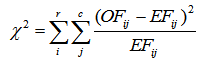
The test statistic for the Pearson chi-square test of independence for a contingency table with *r* rows and *c* columns is calculated as follows (Preacher, 2001):
 (1)
(1)
(45 × 70)/200 = 15.75
(45 × 130)/200 = 29.25
(155 × 70)/200 = 54.25
(155 × 130)/200 = 100.75
The chi-square test is a non-parametric method that quantifies the discrepancy between these observed and expected frequencies to determine if a significant association exists between the variables. A key advantage of this test, like other non-parametric methods, is that it does not require assumptions about the underlying data distribution, equality of variances, or homogeneity (McHugh, 2013; Sharpe, 2015).
To perform the test, the chi-square statistic is first calculated. The degrees of freedom (df) are then determined as (number of rows - 1) × (number of columns - 1). Finally, the calculated test statistic is compared to the critical value from the chi-square distribution table for the corresponding df. If the test statistic exceeds the critical value, the null hypothesis of independence is rejected (Sharpe, 2015).
The test statistic for the Pearson chi-square test of independence for a contingency table with *r* rows and *c* columns is calculated as follows (Preacher, 2001):
(1)Where:
Oij is the observed frequency for the i-th row and j-th column.
Eij is the expected frequency for the i-th row and j-th column.
Σ denotes the summation over all r rows and c columns.
Chi-square test assumptions
The validity of the chi-square test relies on several key assumptions (Turner, 2020):
Oij is the observed frequency for the i-th row and j-th column.
Eij is the expected frequency for the i-th row and j-th column.
Σ denotes the summation over all r rows and c columns.
Chi-square test assumptions
The validity of the chi-square test relies on several key assumptions (Turner, 2020):
- The data must be in the form of frequency counts for each cell.
- The categories of the variables must be mutually exclusive; that is, each observation can belong to only one category of each variable.
- Each subject or case must contribute to one and only one cell in the contingency table.
- The observations must be independent; the value of one observation must not influence another.
- No more than 20% of the expected frequencies should be less than five, and no expected frequency should be less than one. If these conditions are not met, Fisher's exact test is a more appropriate alternative.
Conventional approaches to post-hoc analysis of contingency tables
A significant chi-square test indicates an overall association but does not identify which specific categories contribute to it. To address this, four conventional post-hoc methods have been historically employed for contingency table analysis:
A significant chi-square test indicates an overall association but does not identify which specific categories contribute to it. To address this, four conventional post-hoc methods have been historically employed for contingency table analysis:
- Analysis of standardized residuals
- Partitioning
- Cell comparison
- Ransacking
A brief description of each method is provided below (Fedrizzi and Ferrari, 2018).
-Residual analysis as a post-hoc technique
A long-established method for post-hoc analysis involves the calculation of residuals. A residual is defined as the difference between an observed frequency and its corresponding expected frequency in a contingency table. The magnitude of a residual indicates the cell's contribution to the overall chi-square statistic; a larger residual suggests a greater discrepancy from the null hypothesis of independence (Agresti, 2007). Three common types of residuals are calculated as follows (Agresti, 2013):
- Unstandardized residual for ij- the cell =
OFij – EFij (2)
- Standardized residual for ij- the cell =
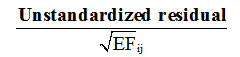 (3)
(3) - Adjusted standardized residual for ij- the cell =
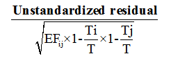 (4)
(4)
In these formulas, EFij denotes the expected frequency for cell (i,j); OFij denotes the observed frequency; Ti is the marginal total for the i-th row; Tj is the marginal total for the j-th column; and T is the grand total of all observations.
As a rule of thumb, standardized residuals are typically interpreted within a range of -2 to +2. A value exceeding an absolute magnitude of 2 suggests that the corresponding cell makes a statistically significant contribution to the overall significance of the chi-square test (MacDonald and Gardner, 2000).
Cell comparison technique
This post-hoc method begins after a significant overall chi-square test is established. It involves selecting pairs of level combinations from the two qualitative variables and performing a statistical test for each pair. The resulting test statistic for a pair is compared to the critical chi-square value for the entire table. A test statistic exceeding this critical value indicates a significant difference in the column proportions between the two levels.
The test statistic in this method is directly influenced by the type of linear contrast used. A contrast is a linear combination of parameters (e.g., column proportions) where the sum of the coefficients is zero (Turner, 2020). Common contrast types include:
-Orthogonal contrasts: A set where the sum of the cross-products of coefficients for any two contrasts is zero (assuming equal sample sizes). A maximum of k-1 orthogonal contrasts are possible for k group means.
-Polynomial contrasts: A specialized subset of orthogonal contrasts used to test for polynomial trends (e.g., linear, quadratic) across ordered means.
-Orthonormal contrasts: Orthogonal contrasts with the additional constraint that the sum of the squared coefficients for each contrast equals one.
For instance, a simple contrast to compare two column proportions would be defined as: Contrast = (1)*P1 + (-1)*P2, where the coefficients sum to zero (1+(-1)=0). The subsequent test statistic can be formulated and summarized using this straightforward contrast.
Test statistics
For a pairwise comparison, a simple contrast can be defined as p1− p2. The test statistic for this contrast is given by:
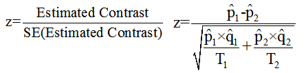 (5)
(5)
In this formula, p1 and p2 represent the estimated proportions for columns 1 and 2, respectively, with qi=1−pi . The terms T1 and T2 denote the marginal totals for columns 1 and 2.
The primary limitation of this post-hoc method is the inflation of the Type I error rate due to multiple comparisons. Furthermore, the results can be sensitive to the specific choice of contrast, which may inadvertently influence the interpretation.
Ransacking post-hoc technique
The ransacking technique involves decomposing a larger contingency table into a series of 2x2 subtables for analysis, rather than comparing all cells simultaneously (Goodman, 1969). A significant challenge with this method, particularly for large tables, is the inflation of the Type I error rate. Conducting multiple statistical tests on these subtables increases the probability of falsely rejecting a true null hypothesis.
Partitioning post-hoc technique
The partitioning method systematically reorganizes an *r* x *c* contingency table into a set of independent, orthogonal 2 x 2 subtables, thereby reducing the dimensionality of the original table. Within these subtables, cells that contribute significantly to the overall association are identified. Various techniques for partitioning exist (Goodman, 1971; Read, 1977).
A key advantage of orthogonal partitioning is that it allows for precise control over the Type I error rate. However, the method has two primary limitations: the number of possible orthogonal partitions is limited by the df of the original table, and many of the resulting partitions may not be substantively meaningful. Furthermore, research indicates that unless comparisons are statistically independent, they cannot be treated as separate and unrelated inquiries, a condition that orthogonal partitioning is designed to meet.
Bonferroni correction for post-hoc analysis of contingency tables
Purpose of the test
In post-hoc pairwise comparisons, the family-wise Type I error rate (alpha) increases with each additional test performed. To control this inflation, an adjustment to the significance level is required (Cabin and Mitchell, 2000). The Bonferroni correction is the most common method for this purpose, which involves lowering the per-comparison alpha level to maintain a desired overall error rate (Goodman, 1969).
The total number of pairwise comparisons CC is determined by the number of column levels being compared. For nn column levels, the number of comparisons is given by C=n(n−1)2C=2n(n−1). The Bonferroni-adjusted significance level αadjαadj is then calculated as:
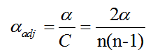 (6)
(6)
The Bonferroni adjustment is applied to the p-values obtained from a series of Z-tests for comparing two independent proportions. The test statistic for each pairwise comparison is calculated as follows:
 (7)
(7)
Where:
p1 and p2 are the observed sample proportions for groups 1 and 2,
n1 and n2 are the sample sizes for the two groups,
p^ is the pooled proportion, calculated as p^=x1+x2/n1+n2, where x1 and x2 are the number of successes in each group.
The Z-test for pairwise comparisons is used to evaluate differences in column proportions across different row levels. In the results presentation, a common practice is to annotate cell counts with letter codes. Cells that share the same letter indicate that their column proportions are not significantly different from one another within the context of the specific row level being compared (Sharpe, 2015).
Z-test for two independent proportions: assumptions
The validity of the Z-test for comparing two independent proportions relies on the following assumptions (Casella and Berger, 2021):
-Sample size: The sample size should be sufficiently large such that the sampling distribution of the proportion is approximately normal. This condition is typically met when n×p>5 and n×(1−p)>5 for each sample, where n is the sample size and p is the proportion.
-Independence: The data points within each group and between the two groups must be independent.
-Randomization: The data should be obtained through a random process, such as simple random sampling.
As a rule of thumb, standardized residuals are typically interpreted within a range of -2 to +2. A value exceeding an absolute magnitude of 2 suggests that the corresponding cell makes a statistically significant contribution to the overall significance of the chi-square test (MacDonald and Gardner, 2000).
Cell comparison technique
This post-hoc method begins after a significant overall chi-square test is established. It involves selecting pairs of level combinations from the two qualitative variables and performing a statistical test for each pair. The resulting test statistic for a pair is compared to the critical chi-square value for the entire table. A test statistic exceeding this critical value indicates a significant difference in the column proportions between the two levels.
The test statistic in this method is directly influenced by the type of linear contrast used. A contrast is a linear combination of parameters (e.g., column proportions) where the sum of the coefficients is zero (Turner, 2020). Common contrast types include:
-Orthogonal contrasts: A set where the sum of the cross-products of coefficients for any two contrasts is zero (assuming equal sample sizes). A maximum of k-1 orthogonal contrasts are possible for k group means.
-Polynomial contrasts: A specialized subset of orthogonal contrasts used to test for polynomial trends (e.g., linear, quadratic) across ordered means.
-Orthonormal contrasts: Orthogonal contrasts with the additional constraint that the sum of the squared coefficients for each contrast equals one.
For instance, a simple contrast to compare two column proportions would be defined as: Contrast = (1)*P1 + (-1)*P2, where the coefficients sum to zero (1+(-1)=0). The subsequent test statistic can be formulated and summarized using this straightforward contrast.
Test statistics
For a pairwise comparison, a simple contrast can be defined as p1− p2. The test statistic for this contrast is given by:
(5)In this formula, p1 and p2 represent the estimated proportions for columns 1 and 2, respectively, with qi=1−pi . The terms T1 and T2 denote the marginal totals for columns 1 and 2.
The primary limitation of this post-hoc method is the inflation of the Type I error rate due to multiple comparisons. Furthermore, the results can be sensitive to the specific choice of contrast, which may inadvertently influence the interpretation.
Ransacking post-hoc technique
The ransacking technique involves decomposing a larger contingency table into a series of 2x2 subtables for analysis, rather than comparing all cells simultaneously (Goodman, 1969). A significant challenge with this method, particularly for large tables, is the inflation of the Type I error rate. Conducting multiple statistical tests on these subtables increases the probability of falsely rejecting a true null hypothesis.
Partitioning post-hoc technique
The partitioning method systematically reorganizes an *r* x *c* contingency table into a set of independent, orthogonal 2 x 2 subtables, thereby reducing the dimensionality of the original table. Within these subtables, cells that contribute significantly to the overall association are identified. Various techniques for partitioning exist (Goodman, 1971; Read, 1977).
A key advantage of orthogonal partitioning is that it allows for precise control over the Type I error rate. However, the method has two primary limitations: the number of possible orthogonal partitions is limited by the df of the original table, and many of the resulting partitions may not be substantively meaningful. Furthermore, research indicates that unless comparisons are statistically independent, they cannot be treated as separate and unrelated inquiries, a condition that orthogonal partitioning is designed to meet.
Bonferroni correction for post-hoc analysis of contingency tables
Purpose of the test
In post-hoc pairwise comparisons, the family-wise Type I error rate (alpha) increases with each additional test performed. To control this inflation, an adjustment to the significance level is required (Cabin and Mitchell, 2000). The Bonferroni correction is the most common method for this purpose, which involves lowering the per-comparison alpha level to maintain a desired overall error rate (Goodman, 1969).
The total number of pairwise comparisons CC is determined by the number of column levels being compared. For nn column levels, the number of comparisons is given by C=n(n−1)2C=2n(n−1). The Bonferroni-adjusted significance level αadjαadj is then calculated as:
(6)The Bonferroni adjustment is applied to the p-values obtained from a series of Z-tests for comparing two independent proportions. The test statistic for each pairwise comparison is calculated as follows:
(7)Where:
p1 and p2 are the observed sample proportions for groups 1 and 2,
n1 and n2 are the sample sizes for the two groups,
p^ is the pooled proportion, calculated as p^=x1+x2/n1+n2, where x1 and x2 are the number of successes in each group.
The Z-test for pairwise comparisons is used to evaluate differences in column proportions across different row levels. In the results presentation, a common practice is to annotate cell counts with letter codes. Cells that share the same letter indicate that their column proportions are not significantly different from one another within the context of the specific row level being compared (Sharpe, 2015).
Z-test for two independent proportions: assumptions
The validity of the Z-test for comparing two independent proportions relies on the following assumptions (Casella and Berger, 2021):
-Sample size: The sample size should be sufficiently large such that the sampling distribution of the proportion is approximately normal. This condition is typically met when n×p>5 and n×(1−p)>5 for each sample, where n is the sample size and p is the proportion.
-Independence: The data points within each group and between the two groups must be independent.
-Randomization: The data should be obtained through a random process, such as simple random sampling.
-Real data: Isfahan Diabetes Prevention Study (IDPS) Cohort
This study utilizes data from the IDPS, a longitudinal cohort study initiated in 2003. The IDPS cohort originally consisted of 3,483 first-degree relatives of patients diagnosed with type 2 diabetes, who were consecutively selected for participation (Abdoli et al., 2021; Safari et al., 2021).
-Example 2: relationship between education level and patient status
This example investigates the association between education level and patient status, where status is categorized as normal, pre-diabetic (Impaired Glucose Tolerance [IGT] or Impaired Fasting Glucose [IFG]), or diabetic. A chi-square test indicated a significant relationship between these two variables (p=0.027), suggesting that the distribution of patient status differs across education levels.
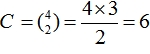
To identify which specific patient status proportions differed significantly between education levels, a post-hoc analysis was performed using pairwise Z-tests with a Bonferroni correction. The column variable (patient status) has 4 levels, resulting in 6 unique pairwise comparisons
( ). The significance level was set at α = 0.05 for the overall family of tests. The results of this Bonferroni-adjusted post-hoc analysis are presented in Table 3.
-Example 2: relationship between education level and patient status
This example investigates the association between education level and patient status, where status is categorized as normal, pre-diabetic (Impaired Glucose Tolerance [IGT] or Impaired Fasting Glucose [IFG]), or diabetic. A chi-square test indicated a significant relationship between these two variables (p=0.027), suggesting that the distribution of patient status differs across education levels.
To identify which specific patient status proportions differed significantly between education levels, a post-hoc analysis was performed using pairwise Z-tests with a Bonferroni correction. The column variable (patient status) has 4 levels, resulting in 6 unique pairwise comparisons
(
). The significance level was set at α = 0.05 for the overall family of tests. The results of this Bonferroni-adjusted post-hoc analysis are presented in Table 3.Table 3: Frequency table of patients’ status and educational level
| Status | P | ||||||
| Diabetic | IFG | IGT | Normal | ||||
| Educational level | Illiterate | Observed Frequencies Expected Frequencies | 14 9.87 |
2 2.80 |
1 5.18 |
4 3.15 |
0.027 Chi-square statistics=18.76 |
| Under diploma | Observed Frequencies Expected Frequencies | 75 70.97 |
21 20.13 |
40 37.25 |
15 22.65 |
||
| Diploma | Observed Frequencies Expected Frequencies | 31 35.72 |
13 10.13 |
21 18.75 |
11 11.40 |
||
| University | Observed Frequencies Expected Frequencies | 21 24.44 |
4 6.93 |
12 12.83 |
15 7.80 |
||
IFG=Impaired fasting glucose; IGT=Impaired glucose tolerance
Therefore, the Bonferroni-adjusted significance level is calculated as follows:
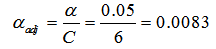
This adjusted alpha (0.0083) was used as the significance threshold for all pairwise comparisons.
The results of the post-hoc analysis (Table 4) revealed specific differences within educational strata. Among illiterate individuals, the proportion of diabetic patients (9.9%, n=14) was significantly higher than the proportion with Impaired Glucose Tolerance (IGT) (1.4%, n=1). Furthermore, within the group with an education level below a diploma, the proportion of diabetic patients (53.2%, n=75) was significantly higher than the proportion with a normal status (33.3%, n=15).
The remaining results can be interpreted similarly, comparing column proportions within each row. It is crucial to note that the significance level for these pairwise tests was not 0.05, but the corrected value of 0.0083.
Table 4: Results of Z- test and adjusted p value by Bonferroni method.
| Final status of individuals | |||||||||
| Diabetes | IFG | IGT | Normal | ||||||
| N | Column proportion | N | Column proportion | N | Column proportion | N | Column proportion | ||
| Education |
illiterate | 14 | 9.9% a | 2 | 5.0% a,b | 1 | 1.4% b | 4 | 8.9% a |
| Under diploma | 75 | 53.2% a | 21 | 52.5% a | 40 | 54.1% a | 15 | 33.3% b | |
| Diploma | 31 | 22.0% a | 13 | 32.5% a | 21 | 28.4% a | 11 | 24.4% a | |
| Upper diploma | 21 | 14.9% a | 4 | 10.0% a | 12 | 16.2% a | 15 | 33.3% b | |
| Total | 141 | 100.0% | 40 | 100.0% | 74 | 100.0% | 45 | 100.0% | |
Each letter denotes a subset of categories whose column proportions do not differ significantly from each other at the 0.05 level.
Software implementation: conducting a Bonferroni post-hoc test
This section provides a practical guide for performing a Bonferroni-adjusted post-hoc analysis following a significant chi-square test in three common statistical software environments: SPSS, Stata and R.
SPSS
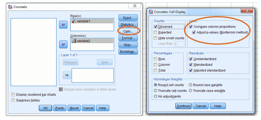
The Bonferroni adjustment is available in the Crosstabs procedure.
This section provides a practical guide for performing a Bonferroni-adjusted post-hoc analysis following a significant chi-square test in three common statistical software environments: SPSS, Stata and R.
SPSS
The Bonferroni adjustment is available in the Crosstabs procedure.
- Navigate to: Analyze > Descriptive Statistics > Crosstabs
- Specify your Row and Column variables.
- Click Statistics and select Chi-square.
- Click Cells. In the "Counts" section, ensure Observed is selected. In the "Z-test" section, check Compare column proportions and select Adjust p-values (Bonferroni method).
- Click Continue and then OK to run the analysis.
Stata
The Bonferroni-adjusted pairwise comparisons of proportions can be performed post-estimation after a tabulate command using the prtest command for each pair in a loop, manually adjusting the alpha level. Alternatively, use the user-written postchi package.
The Bonferroni-adjusted pairwise comparisons of proportions can be performed post-estimation after a tabulate command using the prtest command for each pair in a loop, manually adjusting the alpha level. Alternatively, use the user-written postchi package.
Menu:
Statistics → Summaries, tables, and tests → Classical tests of hypotheses → Proportion test calculator
command:
* Install the postchi package (once)
ssc install postchi
* After a tabulation, e.g., tab rowvar colvar, chi2
postchi, adjust(bonferroni)
Statistics → Summaries, tables, and tests → Classical tests of hypotheses → Proportion test calculator
command:
* Install the postchi package (once)
ssc install postchi
* After a tabulation, e.g., tab rowvar colvar, chi2
postchi, adjust(bonferroni)
R
The chisq.posthoc.test package provides a direct function for this purpose.
# Install and load the package
install.packages("chisq.posthoc.test")
library(chisq.posthoc.test)
# Perform the post-hoc test
chisq.posthoc.test(x, method = "bonferroni")
install.packages("chisq.posthoc.test")
library(chisq.posthoc.test)
# Perform the post-hoc test
chisq.posthoc.test(x, method = "bonferroni")
Conclusion
This tutorial has demonstrated that post-hoc analysis is a critical and applicable step following a significant chi-square test, moving beyond the common perception of its use solely in ANOVA. While several historical methods, such as residual analysis, partitioning, and ransacking, offer ways to interrogate a contingency table, they often lack a straightforward mechanism to control the inflated Type I error rate inherent in multiple comparisons. The pairwise Z-test for proportions, when integrated with the Bonferroni correction, directly addresses this fundamental limitation. By providing a clear, adjustable significance threshold, the Bonferroni method offers a robust and interpretable framework for identifying specific category differences. Consequently, we strongly recommend its adoption for post-hoc pairwise comparisons after a significant chi-square result. This approach ensures statistical rigor while simplifying the interpretation of complex categorical relationships, making it an invaluable tool for researchers across medical and social science disciplines.
Availability of data
The data can be obtained from the corresponding author upon a reasonable request.
Author contributions
FM and MA conceived the concept of this study, carried software code, and wrote the manuscript. Both authors read and approved the final manuscript.
Acknowledgements
The authors would like to express their sincere gratitude to the respected reviewers for their insightful comments and constructive suggestions, which significantly improved the quality of this manuscript. We are also deeply thankful to the Editor-in-Chief, Dr. J. Sadeghizadeh-Yazdi, for his meticulous guidance and for steering the numerical examples of the paper toward the field of nutrition.
Statement
We acknowledge the use of ChatGPT (OpenAI) for the purpose of English language polishing and native-level editing of the manuscript.
Conflict of interests
The authors declare that there is no conflict of interests.
Funding
This research did not receive any specific grant from funding agencies in the public, commercial, or non-profit sectors.
Ethical consideration
Not applicable.
References
Abdoli M., Amini M., Safari S., Aminorroaya A., Feizi A. (2021). Patterns of changes in abdominal obesity indices in prediabetic individuals: Results of a 16-year prospective cohort study among first-degree relatives of type 2 diabetic patients. Iranian Journal of Endocrinology and Metabolism. 22: 441-441.
Agresti A. (2007). An introduction to categorical data analysis. John Willey and Sons, Hoboken, New Jersey. [DOI: 10.1002/ 0470114754]
Agresti A. (2013). Categorical data analysis. 3rd edition. John Willey and Sons, Hoboken, New Jersey. URL: https://www. wiley.com/en-us/Categorical+Data+Analysis% 2C+3rd+Edition-p-9780470463635.
Bahariniya S., Madadizadeh F. (2021). Review of the statistical methods used in original articles published in Iranian Journal of Public Health from 2015–2019. Iranian Journal of Public Health. 50: 1577. [DOI: 10.18502/ijph.v50i8.6803]
Cabin R.J., Mitchell R.J. (2000). To Bonferroni or not to Bonferroni: when and how are the questions. Bulletin of the Ecological Society of America. 81: 246-248.
Casella G., Berger R.L. (2021). Statistical inference. 2nd Edition. Chapman and Hall/CRC, Boca Raton, Florida. URL: https:// pages.stat.wisc.edu/~shao/stat610/Casella_Berger_Statistical_Inference.pdf.
Connelly L. (2019). Chi-square test. Medsurg Nursing. 28: 127-127.
Cox M.K., Key C.H. (1993). Post hoc pair-wise comparisons for the chi-square test of homogeneity of proportions. Educational and Psychological Measurement. 53: 951-962. [DOI:10.1177/ 0013164493053004008]
Fedrizzi M., Ferrari F. (2018). A chi-square-based inconsistency index for pairwise comparison matrices. Journal of the Operational Research Society. 69: 1125-1134.
Goodman L.A. (1969). How to ransack social mobility tables and other kinds of cross-classification tables. American Journal of Sociology. 75: 1-40.
Goodman L.A. (1971). Partitioning of chi-square, analysis of marginal contingency tables, and estimation of expected frequencies in multidimensional contingency tables. Journal of the American Statistical Association. 66: 339-344. [DOI: 10.2307/2283933]
Lachenbruch P.A. (2014). McNemar test. Wiley StatsRef: Statistics Reference Online. [DOI: 10.1002/9781118445112.stat04876]
Laurencelle L. (2021). The exact binomial test between two independent proportions: a companion. The Quantitative Methods for Psychology. 17: 76-79. [DOI: 10.20982/tqmp.17.2. p076]
Liu H., Cui S.W., Chen M., Li Y., Liang R., Xu F., Zhong F. (2019). Protective approaches and mechanisms of microencapsulation to the survival of probiotic bacteria during processing, storage and gastrointestinal digestion: a review. Critical Reviews In Food Science and Nutrition. 59: 2863-2878. [https://www.tandfonline. com/doi/ full/ 10.1080/10408398.2018.1462763]
MacDonald P.L., Gardner R.C. (2000). Type I error rate comparisons of post hoc procedures for I j Chi-Square tables. Educational and Psychological Measurement. 60: 735-754. [DOI: 10.1177/ 00131640021970871]
MacDonald P.L., Gardner R.C. (2000). Type I error rate comparisons of post hoc procedures for I j Chi-Square tables. Educational and Psychological Measurement. 60: 735-754. [DOI: 10.1177/ 00131640021970871]
Madadizadeh F., Bahariniya S. (2022a). Frequency of the statistical methods and relation with acceptance period in archives of Iranian medicine articles: a review from 2015–2019. Archives of Iranian Medicine. 25: 267-273. [DOI: 10.34172/aim.2022.43]
Madadizadeh F., Bahariniya S. (2022b). Statistical methods used in Iranian red crescent medical Journal articles and their relationship with acceptance period: a review from 2014-2021. Iranian Red Crescent Medical Journal. 24.
McHugh M.L. (2013). The chi-square test of independence. Biochemia medica. 23: 143-149. [DOI: 10.11613/BM.2013.018]
Narum S.R. (2006). Beyond Bonferroni: less conservative analyses for conservation genetics. Conservation Genetics. 7: 783-787. [DOI: 10.1007/s10592-005-9056-y]
Preacher K.J. (2001). Calculation for the chi-square test: an interactive calculation tool for chi-square tests of goodness of fit and independence. URL: http://quantpsy.org.
Read C.B. (1977). Partitioning chi-squape in contingency tables: a teaching approach. Communications in Statistics-Theory and Methods. 6: 553-562. [DOI: 10.1080/03610927708827513]
Safari S., Abdoli M., Amini M., Aminorroaya A., Feizi A. (2021). A 16-year prospective cohort study to evaluate effects of long-term fluctuations in obesity indices of prediabetics on the incidence of future diabetes. Scientific Reports. 11: 11635.
Sharpe D. (2015). Chi-square test is statistically significant: now what? Practical Assessment, Research, and Evaluation. 20: 8. [DOI: 10.7275/tbfa-x148]
Turner R.J. (2020). Safe tests for 2 x 2 contingency tables and the Cochran-Mantel-Haenszel test. BNAIC /BeneLearn. 2020: 438. URL: https://enablingpersonalizedinterventions.nl/2020-11-09/ BNAICBENELEARN_2020_Final_paper_13.pdf.
[*] Corresponding author (M. Abdoli)
Email: abdoli_75@yahoo.com
Orchid ID: https://orcid.org/0000-0002-5525-8549
Email: abdoli_75@yahoo.com
Orchid ID: https://orcid.org/0000-0002-5525-8549
Type of Study: Short communication |
Subject:
Special
Received: 24/02/11 | Accepted: 25/04/16 | Published: 25/12/21
Received: 24/02/11 | Accepted: 25/04/16 | Published: 25/12/21
References
1. Abdoli M., Amini M., Safari S., Aminorroaya A., Feizi A. (2021). Patterns of changes in abdominal obesity indices in prediabetic individuals: Results of a 16-year prospective cohort study among first-degree relatives of type 2 diabetic patients. Iranian Journal of Endocrinology and Metabolism. 22: 441-441.
2. Agresti A. (2007). An introduction to categorical data analysis. John Willey and Sons, Hoboken, New Jersey. [DOI: 10.1002/ 0470114754] [DOI:10.1002/0470114754]
3. Agresti A. (2013). Categorical data analysis. 3rd edition. John Willey and Sons, Hoboken, New Jersey. URL: https://www. wiley.com/en-us/Categorical+Data+Analysis% 2C+3rd+Edition-p-9780470463635.
4. Bahariniya S., Madadizadeh F. (2021). Review of the statistical methods used in original articles published in Iranian Journal of Public Health from 2015-2019. Iranian Journal of Public Health. 50: 1577. [DOI: 10.18502/ijph.v50i8.6803] [DOI:10.18502/ijph.v50i8.6803] [PMID] [PMCID]
5. Cabin R.J., Mitchell R.J. (2000). To Bonferroni or not to Bonferroni: when and how are the questions. Bulletin of the Ecological Society of America. 81: 246-248.
6. Casella G., Berger R.L. (2021). Statistical inference. 2nd Edition. Chapman and Hall/CRC, Boca Raton, Florida. URL: https://pages.stat.wisc.edu/~shao/stat610/Casella_Berger_Statistical_Inference.pdf.
7. Connelly L. (2019). Chi-square test. Medsurg Nursing. 28: 127-127.
8. Cox M.K., Key C.H. (1993). Post hoc pair-wise comparisons for the chi-square test of homogeneity of proportions. Educational and Psychological Measurement. 53: 951-962. [DOI:10.1177/ 0013164493053004008] [DOI:10.1177/0013164493053004008]
9. Fedrizzi M., Ferrari F. (2018). A chi-square-based inconsistency index for pairwise comparison matrices. Journal of the Operational Research Society. 69: 1125-1134. [DOI:10.1080/01605682.2017.1390523]
10. Goodman L.A. (1969). How to ransack social mobility tables and other kinds of cross-classification tables. American Journal of Sociology. 75: 1-40. [DOI:10.1086/224743]
11. Goodman L.A. (1971). Partitioning of chi-square, analysis of marginal contingency tables, and estimation of expected frequencies in multidimensional contingency tables. Journal of the American Statistical Association. 66: 339-344. [DOI: 10.2307/2283933] [DOI:10.2307/2283933]
12. Lachenbruch P.A. (2014). McNemar test. Wiley StatsRef: Statistics Reference Online. [DOI: 10.1002/9781118445112.stat04876] [DOI:10.1002/9781118445112.stat04876] [PMCID]
13. Laurencelle L. (2021). The exact binomial test between two independent proportions: a companion. The Quantitative Methods for Psychology. 17: 76-79. [DOI: 10.20982/tqmp.17.2. p076] [DOI:10.20982/tqmp.17.2.p076]
14. Liu H., Cui S.W., Chen M., Li Y., Liang R., Xu F., Zhong F. (2019). Protective approaches and mechanisms of microencapsulation to the survival of probiotic bacteria during processing, storage and gastrointestinal digestion: a review. Critical Reviews In Food Science and Nutrition. 59: 2863-2878. [https://www.tandfonline. com/doi/ full/ 10.1080/10408398.2018.1462763] [DOI:10.1080/10408398.2017.1377684] [PMID]
15. MacDonald P.L., Gardner R.C. (2000). Type I error rate comparisons of post hoc procedures for I j Chi-Square tables. Educational and Psychological Measurement. 60: 735-754. [DOI: 10.1177/ 00131640021970871] [DOI:10.1177/00131640021970871]
16. Madadizadeh F., Bahariniya S. (2022a). Frequency of the statistical methods and relation with acceptance period in archives of Iranian medicine articles: a review from 2015-2019. Archives of Iranian Medicine. 25: 267-273. [DOI: 10.34172/aim.2022.43] [DOI:10.34172/aim.2022.43] [PMID] [PMCID]
17. Madadizadeh F., Bahariniya S. (2022b). Statistical methods used in Iranian red crescent medical Journal articles and their relationship with acceptance period: a review from 2014-2021. Iranian Red Crescent Medical Journal. 24.
18. McHugh M.L. (2013). The chi-square test of independence. Biochemia medica. 23: 143-149. [DOI: 10.11613/BM.2013.018] [DOI:10.11613/BM.2013.018] [PMID] [PMCID]
19. Narum S.R. (2006). Beyond Bonferroni: less conservative analyses for conservation genetics. Conservation Genetics. 7: 783-787. [DOI: 10.1007/s10592-005-9056-y] [DOI:10.1007/s10592-005-9056-y]
20. Preacher K.J. (2001). Calculation for the chi-square test: an interactive calculation tool for chi-square tests of goodness of fit and independence. URL: http://quantpsy.org.
21. Read C.B. (1977). Partitioning chi-squape in contingency tables: a teaching approach. Communications in Statistics-Theory and Methods. 6: 553-562. [DOI: 10.1080/03610927708827513] [DOI:10.1080/03610927708827513]
22. Safari S., Abdoli M., Amini M., Aminorroaya A., Feizi A. (2021). A 16-year prospective cohort study to evaluate effects of long-term fluctuations in obesity indices of prediabetics on the incidence of future diabetes. Scientific Reports. 11: 11635. [DOI:10.1038/s41598-021-91229-9] [PMID] [PMCID]
23. Sharpe D. (2015). Chi-square test is statistically significant: now what? Practical Assessment, Research, and Evaluation. 20: 8. [DOI: 10.7275/tbfa-x148]
24. Turner R.J. (2020). Safe tests for 2 x 2 contingency tables and the Cochran-Mantel-Haenszel test. BNAIC /BeneLearn. 2020: 438. URL: https://enablingpersonalizedinterventions.nl/2020-11-09/ BNAICBENELEARN_2020_Final_paper_13.pdf.
| Rights and permissions | |
 |
This work is licensed under a Creative Commons Attribution-NonCommercial 4.0 International License. |
